|
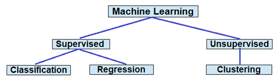
Supervised Learning
|
|
Easiest way to understand supervised learning is -
imagine a new robot such as a autonomous wheelchair
is procured in an airport. Out of the box, it
starts operating freely without supervision, but will
go everywhere and create paths, which may not be the
best approach. To get the best performance from the
robotic wheelchair, an airport technical staff will
using a remote control, walk it to passenger pick up
area and create paths to departure terminals.
Similarly the robotic wheelchair is taught arrival
terminals to drop off locations in
supervised mode. These paths are
saved in the robot's memory, which basically is
training data and the robot is initialized by
supervised learning
for daily usage.
|
| |
|
Now that the robotic wheelchair has the paths
configured, it can now take passengers who
require wheelchair assistance - from check-in to
departing terminals or pick up arriving
passengers and drop them at prerequested
locations. The internal AI and machine learning
algorithms will take care of autonomous
navigation of the wheelchair within the
airport, beep if it requires space to go
forward or sees a obstacle, stop before
colliding with any other object and take
autonomous decisions at other type of new
situation it encounters, still completing
its mission successfully.
|
| |
|
Two Key Categories of Supervised Learning - Classification and Regression
|
| |
|
1. Classification
|
|
Data typically is not classified (raw) to start with.
Classification is the method of converting
unclassified data into classified data
by using ML algorithms.
|
| |
|
Reinforced Learning
|
|
In this type of Machine Learning, a system is allowed
learn on its own. In our case the robotic wheelchair
is made to create paths within the airport by trial
and error methodology. For correct path the robot
is rewarded - achieved some form of
probability/statistical programming
algorithms and it saves the data for future use. This
process is repeated until all possible routes are
created.
|
| |
|
2. Regression
|
|
For two variables x and y, regression
in statistics
represents the dependency of the average value of y on
x. We have the well know
linear regression
equation
|
| |
|
y = mx + c
|
|
where m is the slope and c is the y-intercept.
|
| |
|
Slope and Intercept Computation
(regression functions in languages and SQL)
|
| |
|
COVAR_POP(x, y) = (SUM(x * y) - SUM(y) * SUM(x)/n)/n
|
| |
|
VAR_POP(y) = SUM((xi - AVG(y))2)/n
|
|
where xi represents individual values of x1,
x2, . . . xn
|
| |
|
REGR_SLOPE(x,y) = COVAR_POP(x, y)/VAR_POP(y)
|
| |
|
REGR_INTERCEPT(x, y) = AVG(x) - REGR_SLOPE(x, y) * AVG(y)
|
|
Unsupervised Learning
|
|
Contrary to supervised learning, here is data is collected
with no intention of prediction of a next value. Using machine
learning algorithms, the unlabeled datasets are analyzed and
organized into subgroups or clusters, known as
clustering.
Due to least human intervention in the learning process,
unsupervised learning is best suited for exploratory analysis,
image and pattern recognition, cancer diagnosis, customer
purchase pattern analysis and so on to name a few. One of the
greatest advantages of unsupervised learning is, the
ease in getting unlabeled data.
|
| |
|
Models in unsupervised learning are designed to reduce the
number of features in unlabeled data by the process of
dimensionality reduction. This is achieved by two
key algorithms
PCA
and
SVD.
|
| |
| |
|
Principal Component Analysis (PCA)
|
|
PCA is a dimensionality reduction algorithm used to reduce
dimensions in large unlabeled data. For a series of two
uncorrelated values (x,y), the PCA algorithm can be used to
find a sequence of linear combinations of the variables that
have maximal variance. The two values are the
principal components.
PCA is used for data visualization,
noise reduction to improve data quality and so on.
|
| |

|
|
PCA, Victor Powell [16]
|
| |
| |
|
Singular Value Decomposition (SVD)
|
|
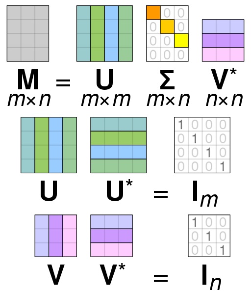
The mathematical definition of
SVD is, it is a matrix factorization of a matrix A[m, n]
with singular values σ1 ≥ σ2
. . . ≥ σn ≥ 0. The index r denotes
singular values of A.
|
| |
|
SVD Matrix:
M = U ∑ V*
|
| |
|
U is an [m, m] orthogonal matrix.
|
|
∑ represents a [m, n] matrix whose
ith diagonal value corresponds to singular
value σi = 1,2,.. r. All other
values are zero.
|
|
V is an [n, n] orthogonal matrix.
|
| |
|
|
Photo: SVD Visualization, Wikipedia
|
| |
| |
| Clustering
|
| Clustering is partitioning of data into subsets or
clusters such that data in a cluster has common characters.
By clustering, common patterns in data, patterns in images
etc. can be easily deciphered. There are several
algorithms used in clustering.
|
| |
|
Clustering Algorithms
|
|
Hierarchical Clustering
|
|
K-means Clustering
|
|
Gaussian Mixture Models (GMM)
|
|
DBSCAN (Density-Based Spatial Clustering of Applications with Noise)
|
|
Agglomerative Clustering
|
|
Spectral Clustering
|
|
Mean Shift Clustering
|
|
Affinity Propagation
|